Dynamic modelling of photosynthesis in marine and
estuarine ecosystems
Running
title: Dynamic modelling of photosynthesis
P. Duarte1 & J. G. Ferreira2
1 Universidade Fernando Pessoa,
Departamento de Ciências e Tecnologia, Praça 9 de Abril, 349, 4200 Porto,
Portugal. E-mail: pmd@mail.fct.unl.pt
2 Universidade Nova de Lisboa, Dept.
de Ciências e Engenharia do Ambiente, Quinta da Torre, 2825 Monte de Caparica,
Portugal. E-mail: joao.imar@mail.telepac.pt
Abstract
The relationship between primary productivity and light intensity is
usually modelled as a static representation of photosynthesis, assuming that
the parameters describing the response to light are constant. However, these
parameters have a dynamic behaviour justifying the development of dynamic
models in order to improve the description of photosynthesis in the sea.
In this work a mathematical model is used to simulate several situations
where the phytoplankton exposure to light is controlled by the temporal
variation of light intensity and the vertical advective and diffusive flux. The
model includes both a static and a dynamic description of photosynthesis. It
uses object-oriented methods to switch between different types of productivity
response to light intensity and to potential photoinhibition effects.
The main conclusions emerging from the simulations performed are that
the dynamic behaviour of the production-light curves is relevant in the
simulation of primary productivity, and that this relevance is more pronounced
under high light conditions and/or in the absence of vertical mixing. It is
suggested that large scale models, where the time and spatial scales are too
large to include the dynamic behaviour of the photosynthetic light response,
may be parameterized by smaller scale simulations including the mentioned
dynamic behaviour.
Keywords
Ecological
model, phytoplankton, productivity, mixing, dynamic simulation, OOP
Introduction
During the last decades a considerable amount of research has been
carried out on primary productivity modelling (e.g. Steele, 1962; Vollenweider,
1965; Jassby and Platt, 1976; Platt et al., 1980; Fasham and Platt, 1983;
Eilers and Peeters, 1988). In most of these works formulations of the
relationship between primary productivity and light intensity were proposed and
tested against field and/or laboratory data. Most of these equations are
empirical, only a few of them being deduced from the physiology of
photosynthesis (e.g. Fasham and Platt, 1983; Eilers and Peeters, 1988). These
formulations have been used for several years in ecological models.
The productivity-light (P-I)
relationships can be divided into static and dynamic. In the former it is
assumed that the parameter values, e.g. the maximum production rate (Pmax), the optimal light
intensity (Iopt), etc.,
are constant, whilst in the latter these parameters are recalculated as a
function of light intensity and/or some other forcing functions. The static
formulations are by far the most widely used. Only in a few cases were dynamic
formulations used in ecological models (Falkowski and Wirick, 1981; Pahl-Wostl
and Imboden, 1990; Janowitz and Kamykowski, 1991). This may probably be
accounted for by the greater number of parameters required for dynamic
representation and the increased complexity in its formulation.
Important information regarding the dynamic aspects of photosynthesis
has been provided through experimental work (e.g. Marra, 1978; Neale and Marra,
1985; Falkowski and LaRoche, 1991). It is now clear that the parameters used in
the productivity-light curves change over time as a result of adaptation at
different time scales. It is also known that the classical way of measuring
primary productivity by the light/dark bottle technique, and the use of the
results obtained to estimate the P-I
curve parameters may lead to overestimation of photoinhibition (Lewis et al., 1984; Gallegos and Platt, 1985;
Pahl-Wostl and Imboden, 1990). This is illustrated in Fig. 1, which shows model
results (see below) of productivity versus light intensity after algae were
exposed for various periods of time to a critical (inhibition) light level.
During the day, algal photosynthesis closely follows the variation in
light intensity until a frequency of 10 cycles hour-1, under cloudy
sky or variable light (Marra and Heinemann, 1982). Above a certain light level
the correlation between productivity and light decreases due to the
nonlinearity of the P-I relationship
(Marra and Heinemann, 1982). When light intensity remains very high for a long
time photoinhibition becomes more and more important. Noon or afternoon
depression seems to occur as a result of photoinhibition (e.g. Marra, 1978;
Pahl-Wostl and Imboden, 1990).
The measurement of integral photosynthesis in the mixed layer, estimated
from light/dark bottle experiments, when the bottles were suspended at fixed
depths and when the bottles were moved vertically though the mixed layer, gave
higher results in the latter case (Marra, 1978). The observed differences were
significant when the light intensity at surface was above the critical values
for photoinhibition. In this case the algae in the fixed bottles experienced
photoinhibition, whereas those in the moving bottles were not exposed to a
critical light long enough to experience photoinhibition. This experiment
showed the importance of considering vertical movement and light variability
when simulating primary productivity in the mixed layer. However, according to
the previous author, the observed differences could not be explained solely by
photoinhibition.
These differences could be increased due to the physiological adaptation
to light, leading to different initial slopes and Pmax values for the P-I
relationship. During the night algae become shade-adapted, and exhibit a higher
photosynthetic efficiency at low light (higher initial slope). During the day,
they tend to become light-adapted due to (among other things) a decrease in the
initial slope. By the end of the day, when light intensity becomes lower, they
tend to shade-adapt again (Falkowski and Wirick, 1981). These authors simulated
the light and shade adaptations using the chlorophyll:carbon ratio, showing
that light-adapted algae have a lower ratio than shade-adapted ones.
In some of the studies referred, special care was taken to simulate
photoinhibition as a time-dependent parameter (e.g. Pahl-Wostl and Imboden,
1990; Janowitz and Kamykowski, 1991). In other studies, special care was taken
to simulate the light and shade adaptation (e.g., Falkowski and Wirick, 1981).
Both Falkowski and Wirick (1981) and Janowitz and Kamykowski (1991) simulated
sunlight variability and vertical movement. However, in none of these studies
were all the dynamic aspects mentioned above considered together, and their
relative importance analysed in relation to real ocean or coastal situations.
The diagram shown in Fig. 2 synthesises the links between various
physical and biological phenomena that influence the primary productivity
parameters. As demonstrated earlier
(Lewis et al., 1984; Gallegos and Platt, 1985) the time scale of mixing
is of crucial importance in the development of photoadaptation and inhibition,
because it determines the time that the phytoplankton spends at each depth
under a certain light regime. In order to consider the connections between all
the compartments shown in Fig. 2, and their variability, it is necessary to
employ a mathematical model. It is important to consider the mixing events not
only as the determining factor of the time phytoplankton spends at various
depths, but also as the process through which differently adapted phytoplankton
mixes at various depths, resulting in changes to the P-I population parameters.
The objectives of the present work were:
·
To
develop a model for primary production which takes into account the various
aspects of the dynamics of the P-I
curve parameters;
·
To
couple the biological model with a physical model to simulate vertical
exchange, not only of variables but also of population parameters;
·
To
examine the sensitivity of primary production models to the dynamics of the P-I curve parameters.
In order to achieve these objectives, the simulation of phytoplankton
productivity was carried out for two cases: A mixed water column and a
perfectly stratified water column. In the mixed case, the physical model was
used to simulate vertical transport. Gross productivity was calculated as a
function of light intensity.
Methodology
A description of the model concepts and implementation is given below.
This is divided into 4 sections: Physical
modelling, biological modelling, linkage, and implementation. Finally, details of the different model simulations
carried out are indicated.
Physical
modelling
Light
intensity and water temperature
Light intensity is used as a forcing function both for the physical and
the biological model. In the physical model, light intensity influences water
temperature and therefore water density. In the biological model, the
photosynthetically active radiation (PAR) forces primary productivity.
Estimation of light intensity and radiation fluxes between the sea and the
atmosphere was based on standard formulations described in Brock (1981) and
Portela and Neves (1994).
Hydrodynamics
The hydrodynamic model used in this work was described by Price (1986)
and has been applied by Janowitz and Kamykowski (1991) to Lake Titicaca. It is
a one-dimensional vertical exchange model, forced by the wind stress at the
surface, by the solar and long wave radiation and, by the sensible and latent
heat transfers across the surface. The number of vertical layers is variable;
in the present case 20 layers of 3 m depth were considered, for a 60 m water
column.
The model has three stages (or phases):
(i) A deterministic stage, which uses the wind stress forcing at the
atmosphere-ocean interface in order to calculate the velocity of the surface
layer, and which calculates the density of all the layers based on incident
radiation. Although salinity is a model state variable, it is not considered in
the density determination because the vertical density structure of the water
column is considered to be mainly temperature dependent.
(ii) A convective mixing stage, which looks for vertical instability in
the water column. This stage uses a stepwise approach, examining adjacent
layers for densimetric instability, and re-initialising all the boxes above
with the average values for the horizontal velocity components and density.
(iii) A dynamic mixing stage, which is responsible for turbulent mixing
between layers based on the shear stress at the interface. This is calculated
by means of the Richardson number obtained for each layer.
Biological
modelling
Static
versus dynamic approaches
The biological model simulates phytoplankton biomass and productivity.
In all model simulations all physiological and demographic phytoplankton
processes were computed in the same manner, with the exception of productivity.
Respiration was computed as a fixed fraction of primary productivity
during daylight (30 %) and at a fixed rate during night hours (10 % of the
maximal production rate). Exudation was computed as a fixed fraction of
productivity (10 %). Mortality was computed as a fixed rate (0.05 day-1).
The initial biomass was assumed to be 1 mg chl l-1. All these
values are well within the ranges reported in the literature (see Jørgensen et al., 1991). Biomass changes were
computed from the sum of all gain and loss processes including biomass
exchanges between the model boxes.
Primary productivity modelling was carried out by means of static and
dynamic formulations. In the former, the productivity model parameters remained
constant over the simulation period, whereas in the latter parameters were
changed as a function of the phytoplankton light history and mixing events. The
model parameters were considered at the population level, not at the individual
level.
The model described in Eilers and Peeters (1988, 1993) (1) was used to
simulate productivity (P) as a
function of light intensity (I). This
model was chosen because it is based on the physiology of photosynthesis. An
added advantage is that the depth integration of the model equation has an
analytical solution (Eilers and Peeters, 1988).
![]() (1)
(1)
By differentiating (1) Eilers and Peeters (1988) expressed the usual
characteristics of the P-I curves,
namely the initial slope (S), the maximal production rate (Pmax) and the optimal light
intensity (Iopt) as a
function of the parameters a, b and c:
![]() (2)
(2)
![]() (3)
(3)
![]() (4)
(4)
Following these authors the reverse equations are:
 (5)
(5)
 (6)
(6)
![]() (7)
(7)
Initial values for a, b and c were chosen from literature data on Pmax, Iopt
and S (see Jørgensen et al., 1991). A Pmax of 0.15 h-1, an Iopt of 400 mE m-2 s-1 and
an S of 4 X 10⁻⁷ mE m-2 were chosen. These values
correspond to an a of 0.01, a b of 3.16 and a c of 735.76.
Some changes to Eilers' model
were introduced in order to account for the dynamic aspects of its parameters.
These changes consisted in:
i)
Recalculating
the photoinhibition parameter a as a
function of exposure time to a critical light intensity (above the optimal
light level);
ii)
Recalculating
the parameters a, b and c as a function of the changes in the initial slope (photosynthetic
efficiency);
iii)
Recalculating
the parameters a, b and c as a function of the changes in the initial slope, and the
parameter a also as a function of
exposure time to a critical light intensity.
Model simulations were carried out keeping the parameters constant or
recalculating them according to each of the changes indicated. Hereafter we
will use the term “Static phytoplankton” when referring to simulations carried
out by keeping the P-I model
parameters constant, “Dynamic phytoplankton”, “Adaptative phytoplankton” and
“Dynamic adaptative phytoplankton” when referring to simulations where the
parameters change according to (i), (ii) and (iii), respectively.
The first type of dynamic approach was based on the model DYPHORA
described in Pahl-Wostl and Imboden (1990). Photoinhibition is calculated as a
function of exposure time to light intensity above a critical level.
![]() (8)
(8)
a(t) is the parameter a expressed as a function of time, t is the time exposure to a light intensity above Iopt and ti the light inhibition decay time. The value
for a in the second member of (8)
corresponds to fully developed photoinhibition. According to Pahl-Wostl and
Imboden (1990) ti may
range between 0.5 and 1.5 hours. In the present work ti was considered to be 1 hour. It was also assumed that the recovery from photoinhibition
takes the same time as the development of inhibition (1 hour in the present
case). Recovery is also calculated by (8), except that t becomes the time under a sub-critical light level after the last
exposure to a critical light intensity.
Any change in a causes inverse
changes in Pmax and Iopt (see 3 and 4) unless
there are appropriate changes in b
and c, which was not the case in this
first type of approach. S is not
affected since it depends only on c
(2).
The second dynamic approach was based on the model of Falkowski and
Wirick (1981). In this model the initial slope is calculated as a function of
the chlorophyll: carbon ratio. This ratio changes according to an adaptation
law of the type
![]() (9)
(9)
Where R is the chl:carbon
ratio of the cells, Rw is
the chl:carbon ratio towards which the cells adapt and g is a kinetic coefficient with a
value of 0.2 h-1 during daylight and zero at night, according to
these authors. Shade-adapted phytoplankton have higher chl:carbon ratios than
light-adapted (Falkowski and LaRoche, 1991). The relationship between Rw and incident light is the
same as the one described in Falkowski and Wirick (1981):
![]() if I /
In < 0.01 else
if I /
In < 0.01 else
![]() (10)
(10)
In - Surface incident PAR at noon.
In their model Falkowski and Wirick (1981) used a Michaelis-Menten
function to calculate productivity as a function of light intensity. By
differentiating a Michaelis-Menten P-I
model (11) with respect to light and then determining the limit when light
intensity (I) tends to zero, equation
12 is obtained.
![]() (11)
(11)
k - Half
saturation light intensity.
![]() (12)
(12)
Falkowski and Wirick (1981) computed the half saturation constant as a
function of R:
![]() (13)
(13)
By combining (12) with (13) an
expression for the initial slope as a function of R can be obtained:
 (14)
(14)
In this study the chl:carbon ratio was computed from the integration of
(9) and then the initial slope from (14). Finally the parameters a, b
and c of (1) were recalculated at the
end of each time step using (5), (6)
and (7) after introducing the new value for S.
The values for Pmax and Iopt were kept constant in
the calculations.
The third dynamic approach was a synthesis of the first two. In this
case both the time development of photosynthesis and the chl:carbon ratios were
taken into account to recalculate the model parameters. This recalculation
therefore implied changes in Pmax
and Iopt as in the
first simulation and in S as in the
second simulation. The value of a
used in (8) was taken from (5) after recalculating the slope as in the previous
approach.
Linkage
between physical and biological modelling
The linkage between the physical and the biological model ensures the
vertical transport of phytoplankton. In the simulations where the P-I curve parameters were assumed constant (Static phytoplankton) biomass was
the only phytoplankton attribute that was exchanged between model boxes. In the
other simulations, the P-I curve
parameters were also “exchanged”. In this case an approach similar to that
of Janowitz and Kamykowski (1991) was
followed and a biomass-weighted mean of the parameters was computed whenever
exchange occurred between any two boxes.
Vertical turbulence influences the population model parameters by
putting together phytoplankton with different light histories. For example, if
dark-adapted cells are transported to the surface where light-adapted cells
dominate, the resulting “population” will behave in some intermediate way until
the dark-adapted fraction becomes also light-adapted.
Model
implementation
The coupled physical-biological model was implemented using an
object-oriented (OOP) approach by means of the EcoWin software (CEC, 1994; Ferreira, 1995). A brief description is
given below.
EcoWin uses OOP to relate a set of "ecological" objects by
means of a server, or shell, which effectively allows these to interact with
each other, and displays the results of their interaction. Both the EcoWin shell and the different objects
have been implemented in C++ for WindowsTM.
The advantages of using OOP for ecological modelling are, on the one
hand, the ease of development and flexibility associated with the modularity,
inheritance and polymorphic properties of objects themselves, and on the other,
the much greater conceptual approximation between natural ecosystems and
interacting objects, relative to conventional structured programming methods.
The ecological objects encapsulate attributes (or properties) with
methods which act on these. Thus an object can be conceptually thought of as an
actor whose actions (methods) are governed by its characteristics (attributes);
phytoplankton, for instance, has as one of its attributes a standing crop and
as one of its methods productivity.
OOP is implemented as a set of class hierarchies, such that descendants
inherit ancestor attributes and methods, and may in turn modify the inherited
properties; for instance, diatoms will inherit the properties of the
phytoplankton ancestor and extend them in order to require silica for growth.
The schema developed for this work is presented in Fig. 3, which shows 4
forcing function objects (wind, light, air and water temperature) and 3 base
classes for state variable objects (transport, producers and suspended
particulate matter ). Some of the latter classes are extended (e.g. producers)
into the derived "grandchildren" used for the phytoplankton
simulations (static, dynamic, adaptative and dynamic adaptative classes).
Objects may be switched on or off,
which parallels their existence (or importance) within a system. The analysis
of the model's sensitivity to different components may be much more easily
studied by altering the characteristics of the ecosystem.
EcoWin thus
strikes a balance between a complete "packaged software" approach
(e.g. StellaTM), which will not easily lend itself to extensions to
code, and a first or second generation modelling approach. In the first case,
usage is simplified, but limitations arise as the complexity of the simulated
system increases. In the latter case, many changes can be effected, but
interaction with the user is normally tedious, and modifications usually
require a profound understanding of the code, accompanied by extensive
debugging.
Unfortunately, the latter approach
tends to mean that the user-base of models is frequently very restricted, which
does little to diversify the knowledge sources of different processes involved
in ecological modelling, which must by nature be interdisciplinary .
Model
simulations
Model simulations were carried out to analyse two case-studies, one for
clear ocean water (extinction coefficient - 0.1 m -1) and a second
for turbid water (extinction coefficient - 2 m -1) corresponding to
inshore or estuarine conditions. In each of these case studies two hydrodynamic
conditions were considered, one with vertical wind induced mixing and other without
vertical mixing. For each of these two situations simulations were carried out
with the four phytoplankton objects described above. In synthesis, there are 2
case studies X 2 hydrodynamic conditions X 4 phytoplankton objects, giving a
total of 16 model simulations. A latitude of 44o 47' was considered
for the radiation forcing. All the simulations were performed between julian
day 120 and 125, in order to reproduce spring conditions. In those simulations
with wind forcing a constant wind speed of 10 m s-1 was used. The
model time step was chosen to be 0.05 h after the spatial step was set to 3 m,
following the method described in Janowitz and Kamykowski (1991).
Results
and discussion
In Fig. 4 the evolution of the mixed layer depth for each of the case
studies is shown. As expected, mixing reaches deeper layers when the extinction
coefficient is lower, because light energy penetrates deeper, homogenising the
temperature and therefore decreasing the water column stability.
In the present simulations, the wind velocity considered was sufficient
to mix the water down to a depth below the euphotic depth (c.a. 45 m in the
clear water simulations and 3 m in the turbid water ones, assuming the euphotic
depth to correspond to 1 % of surface incident light (Parsons et al., 1984))
during the simulation period.
Clear ocean water
In Fig. 5 the average gross productivity as a function of depth obtained
with all simulations is shown. It is seen that the differences between the various
model simulations are more pronounced at the surface. The results obtained with
the Dynamic phytoplankton between the surface ant the 12 m depth are higher
than those obtained in any of the other simulations.
The reason for the lower near-surface productivity values of the Static
and the Adaptative phytoplankton in comparison with the Dynamic phytoplankton
is that in the latter, photoinhibition is calculated as a function of time,
therefore it does not have such a negative influence on productivity for the
same amount of time as in the former cases. Pmax
also increases with a decrease in a
as can be seen from (4). This implies that if the phytoplankton is exposed to a
critical irradiance for a short period of time, primary productivity may be higher
than expected when measured for the same light intensity, after the incubation
of the phytoplankton for a period of a few hours (see fig. 1). This has been
observed experimentally (e.g. Marra, 1978) and in the dynamical analysis of
production-light models (e.g. Pahl-Wostl and Imboden, 1990; Eilers and Peeters,
1993).
At greater depths the differences between the average production rates
using Dynamic and Static phytoplankton disappear completely. This is because
there is no photoinhibition and the initial slope is independent of parameter a (see Fig. 1) depending only on c (2). The Adaptative phytoplankton
exhibits greater production rates at greater depths due to dark adaptation
through the increase in the chl:carbon ratios and therefore in the initial
photosynthetic efficiency at low light (see also Figs. 7 and 8 and equations 9,
10 and 14).
The Adaptative phytoplankton shows lower surface values than the Static
phytoplankton. This is a result of the reduction in the chl:carbon ratio and
therefore of the photosynthetic efficiency (initial slope) under high light
intensities near the surface. As is discussed by Eilers and Peeters (1988) the
relative strength of photoinhibition can be estimated from
![]() (15)
(15)
If the slope decreases as occurs near the surface then b will decrease, whereas a and c will increase, therefore decreasing w. As demonstrated by these authors, smaller values of w mean stronger photoinhibition. From
this it is clear why surface phytoplankton tends to be more photoinhibited when
the initial slope is calculated as a function of light.
The lowest near surface results obtained with the Dynamic adaptative
phytoplankton are a result of both an increase in the photoinhibition due to
the reasons just described and a decrease in Pmax. In the case of the Adaptative phytoplankton, among
the P-I curve characteristics only
the slope was changed. However in the case of the Dynamic adaptative
phytoplankton both the slope and Pmax
were changed. This last parameter was recalculated by (4). Any negative change
in the slope causes an increase in a
and c which will cause a reduction of
the production rates and also of Pmax.
The opposite effect at greater depth explains the highest productivities
obtained with the Dynamic adaptative phytoplankton in comparison with all the
other simulations.
The comparison of the simulations carried out with and without vertical
mixing reveals that vertical mixing enhances the productivity at the
near-surface depths, whereas an opposite trend is found in the deeper layers.
The reason for this is that mixing reduces photoinhibition and/or prevents
large decreases in the initial slope near the surface by reducing the time
exposure of phytoplankton to high light levels. However, at the same time
mixing transports photoinhibited and/or light-adapted phytoplankton to deeper
layers, changing the population parameters and therefore reducing productivity.
In all simulations some surface inhibition is apparent, except in the
one obtained with the Dynamic adaptative phytoplankton with hydrodynamics,
where a strange pattern with sub-surface inhibition was obtained. This is a
result of the combination of changes in the photosynthetic parameters induced
both by the light field and the exchange of phytoplankton among the different
layers.
In Fig. 6 the average biomass predicted by all model simulations within
the euphotic depth is shown. It is clear that the differences in the production
rates obtained led to important differences in biomass produced, in spite of the
short time scale of the model runs. The
simulations with vertical mixing included led to less biomass than those
without mixing. This is because mixing dilutes the larger biomass attained near
the surface by transporting part of it to the deeper layers. The Dynamic and
the Dynamic adaptative phytoplankton produced much more biomass than all the
others. Even the Dynamic phytoplankton with mixing produced more biomass than
the Static phytoplankton without mixing.
It the real world there are many mechanisms that influence the
hydrodynamics and biomass production and that were not considered here. For
example, the effect of self-shading could help to control the biomass increase
and to stabilise the water column. Other effects like nutrient limitation, phytoplankton
sinking and zooplankton grazing could also help to control the biomass
increase. These aspects were not considered in order to keep the model as
simple as possible, to be able to demonstrate better the differences of
simulating phytoplankton productivity with static and dynamic formulations
within a mixed layer. The biomasses predicted under the different model
simulations should not be seen as an attempt to simulate reality but as a way
to demonstrate that the differences obtained in productivity reflect large
differences in terms of biomass growth potential.
In Figs. 7 and 8 the changes in the chl:carbon ratio with and without
mixing are shown. The mixing case shows less variability than the non-mixed
one. Water column stratification contributes to increase phytoplankton
adaptation to low or high light. The minimal chl:carbon values are observed
approximately at noon, whereas the maximal values are observed at the beginning
of the daylight period as expected (Falkowski and Wirick, 1981).
Turbid water
In turbid water the model results show some differences by comparison
with the previous set of simulations, but the general patterns are similar.
Photoinhibition is not apparent in fig. 9, because the high turbidity and the
maximal average production rates were obtained at the surface layer. The
Dynamic and the Dynamic adaptative phytoplankton exhibited the largest
productivities.
The biomass variation is shown in Fig. 10. The biomasses produced by the
Dynamic and Dynamic adaptative phytoplankton without hydrodynamics are
considerably larger than the biomasses produced by the Static and Adaptative
phytoplankton without hydrodynamics. With hydrodynamics the differences between
the predicted biomasses are very small.
Regarding the chl:carbon ratios the daily patterns observed are similar
to those described before for clear waters (Figs. 11 and 12).
Reflection
It is very important to measure and simulate accurately primary
production because of its importance as the first link in most trophic chains.
It is well established that the physiological parameters that control the
responses of organisms to environmental conditions are not constant, but change
as a result of adaptation to variable physical and chemical conditions. This
means that the way a particular plant responds to light, for example, is not always the same (Falkowski and
LaRoche, 1991). Similarly, if one studies the activity of an animal, for
example a suspension-feeder bivalve, the parameters that control the
physiological processes are time and space variable (Bayne, 1993). However, in
most mathematical models the physiological parameters are assumed as constant.
The following may be some of the reasons for this assumption:
·
Lack
of knowledge about the dynamics of these parameters;
·
In
many cases the models are designed to work with a time and spatial resolution
that is far to large to simulate dynamically the physiological parameters.
The focus of this work resides in a systematic comparison between
primary production models that include static or dynamic representations of
some parameters. The results obtained with both types of representations give
some insight into the importance and consequences of including/ignoring the
dynamic behaviour of the parameters. This work is an attempt to follow the
emerging idea of developing a new generation of ecological models in which the
parameters taken until know as constants have a dynamic behaviour (Jørgensen,
1992).
Conclusions
The model simulations included static and dynamic approaches to primary productivity
computation. The latter included two types of dynamics: One related to the
developing time of photoinhibition and other related to the light/dark
adaptations. Photoinhibition has a time-scale ranging from 0.5 to 2 hours,
whereas light/dark chl:carbon adaptations have a time-scale of approximately
half a day.
In this work an effort has been made to synthesise in one model current
knowledge on dynamic aspects of photoinhibition and light/dark adaptations. In
the literature there are several models which include dynamic aspects of
photosynthesis (e.g. Falkowski and Wirick, 1981; Neale and Marra, 1985; Denman
and Marra, 1986; Geider and Platt, 1986; Pahl-Wostl and Imboden, 1991) but a
choice was made for those where parameter values existed and in which all the
dynamic aspects that were analysed could be combined.
The model was elaborated as simply as possible, to investigate solely
the importance of dynamic processes under different light and mixing
conditions. The only biological compartment was phytoplankton and other
processes such as nutrient or temperature limitation were not considered. These
conditions allowed the simulation of a phytoplankton population growing
exponentially for a period of 5 days. The final biomass concentrations obtained
under all model simulations were very high. However, similar values were
observed in highly eutrophic areas such as the Adriatic sea (see e.g. Dippner,
1993).
From the results obtained it seems apparent that when the developing
time of photoinhibition is taken into account the surface production rates tend
to be higher, even in very turbid waters. The significance of these differences
may be arguable if one consider the large measurement errors of primary
productivity estimates in the open sea. However, the possible bias introduced
in the computations by neglecting the dynamic aspects of photoinhibition seems
to have a large influence in biomass prediction and therefore in areal
productivity estimates.
Another important fact to retain is that when vertical mixing is
considered, photoinhibition may be present at higher depths than without
mixing, although surface inhibition is weaker than when mixing is absent
(Fig.5). This is a result of the downward transport of partially or fully
inhibited cells. This fact stresses the importance of simulating vertical
transport within the mixed layer and may play an important role in describing
the production curve as a function of depth.
It is interesting to note that under turbid conditions the biomass
predictions obtained under the different simulations are much closer when
vertical wind-induced mixing is present. The differences are still large but
masked by the graph scale. Considering that usually in the high turbidity
areas, like estuaries, the vertical motion depends not only on the wind but
also on the tidal currents and river flow, it is likely that for well mixed
estuaries it is not as important to include the dynamic aspects of
photoinhibition in primary productivity models as is the case for clear waters.
However, the dynamic aspects should be considered whenever possible. In fact,
it may be speculated that these aspects could help to understand why in very
turbid waters a positive carbon balance is possible (Cole et al., 1992).
In a recent work, Kromkamp and Peene (1995) could not obtain a net
phytoplankton growth for the Schelde Estuary with their primary productivity
formulation based on a static formulation, unless they used unrealistically low
respiration rates. It is possible that those results would improve by using a
dynamic approach.
The results from the model runs stress the importance of redesigning the
way primary productivity is usually measured by incubating water samples with
phytoplankton for several hours at fixed depths. After incubation, productivity
is inferred from carbon consumption or oxygen production. The incubation time
is dictated by the detection limit of the measurement method. It is predictable
that under high light intensity, phytoplankton will become inhibited in the
proportion of its exposure time. If the exposure time in the experiment is
larger than the exposure time experienced by phytoplankton under the current
mixing conditions, the measurements will be biased. Thus, it might be
preferable to circulate the incubation flasks through different depths during
the incubation period in order to simulate the mixing events (as in Marra,
1978) or to concentrate phytoplankton in the incubation flasks, to reduce the
incubation period by increasing the consumption/production of carbon/oxygen.
The results obtained with the Adaptative phytoplankton indicate that
changes in the chl:carbon ratios as modelled in the present work do not have a
great influence in the model results when compared to the Static phytoplankton,
except in the clear water case with no mixing. However, the explicit simulation
of the chl:carbon ratio is very important because it may help to resolve one of
the “classical” problems in converting units in ecological models. The large
amplitude of this ratio influences the conversion from chlorophyll to carbon
and vice-versa. These conversions will therefore influence the chlorophyll and
carbon pools and also the links with higher trophic levels.
It is expectable to obtain similar patterns to those obtained in this
study in the analysis and simulation of benthic primary producers. In this
case, instead of the vertical motion of the individuals, the tide induced
vertical motion of the surface must be considered as a factor that will
permanently change the light environment at the bottom. Below a certain depth
this may prevent the development of photoinhibition and therefore may lead to
higher production rates than expected if the time development of photoinhibiton
is not considered.
The conclusions of this work should take into account the simplicity of
the model. It is possible that if other processes and state variables were
included some of the differences between the different model simulations could
be masked, reason why in this study the model was made as simple as possible.
The following points synthesise the conclusions of the present study:
·
The
dynamic behaviour of the production-light curves is relevant in the simulation
of primary productivity;
·
This
relevance is more pronounced under high light conditions and/or in the absence
of vertical mixing;
·
The
dynamic behaviour of the P-I curve
parameters should be included in ecological models whenever possible;
·
In
large-scale models a possible approach could be the parameterization of the
average values for the mentioned parameters, through time and space integration
of the results obtained with smaller scale models.
Target
audience
The conclusions of this work are relevant for anyone working on primary
production and ecological modelling. The EcoWin software is applicable for any
aquatic ecosystem.
Utility
It is clear that in large scale ecological models it is not reasonable
(and almost impossible due to required computing time) to use the time and
spatial scales of the present work. However, it is possible to use the model
described here to integrate over time and space those photosynthetic parameters
that were simulated in this study. This could be a way to parameterize the
large scale models. For example if it was necessary to develop a three
dimensional ecological model for a certain oceanic area, it would be possible
to run the model presented here at several points within the larger domain of
the 3D model with different wind and radiation forcing, characteristic of
different seasons and areas, and then calculate the average values of the above
mentioned parameters. These values could then be used in the larger model.
Alternatively, time series could be obtained for each of the parameters to be
used afterwards in the larger model.
Impact
Based on the conclusions of this work, it is likely that many primary
production estimates, obtained through the assumption of a static behaviour of
the photosynthetic parameters in response to light, may underestimate the real
values. This potentially leads to erroneous conclusions concerning the real
importance of primary producers in the global carbon cycle, and the capacity of
the base of the food chain to support higher trophic levels.
Acknowledgements
This work was supported by EU Environment project EV5V-CT92-0215,
"MARE - Microalgae of the Adriatic Region", and by EU Concerted
Action AIR3-CT94-2219 "Trophic capacity of coastal zones for rearing
oysters, mussels and cockles".
References
[1] J.H.
Steele, Limnol.
Oceanogr. 7 (1962), 137.
[2] R.A. Vollenweider, Mem. Ist. Ital. Hidrobiol. 18 (Suppl.) (1965), 425.
[3] A.D. Jassby and T.Platt, Limnol. Oceanogr 21 (1976), 540.
[4] T. Platt, C.L.Galeggos and W.G.Harrison, J.
Mar. Res. 38 (1980), 687.
[5] M.J.R. Fasham and T. Platt, Proc. R. Soc. Lond.
B219 (1983), 335.
[6] P.H.C. Eilers and J.C.H. Peeters, Ecol.
Modelling 42 (1988) 199.
[7] P.G. Falkowski and C.D. Wirick, Mar. Biol. 65
(1981) 69.
[8] C. Pahl-Wostl and D.M. Imboden, J. Plankton
Res. 12 (1990) 1207.
[9] G.S. Janowitz and D. Kamykowski, J. Plankton
Res. 13 (1991), 983.
[10] J. Marra, Mar. Biol. 46 (1978) 203.
[11] P. Neale and J. Marra, Mar. Ecol. Prog. Ser.,
26 (1985), 113.
[12] P.G. Falkowski and J. LaRoche, J. Phycol. 27
(1991) 8.
[13] M.R. Lewis, J.J. Cullen and T. Platt, Mar. Ecol.
Prog. Ser. 15 (1984), 141.
[14] C.L. Gallegos and T. Platt, Mar. Ecol. Prog.
Ser. 15 (1985), 125.
[15] J. Marra and K. Heinemann, Limnol. Oceanogr. 27
(1982), 1141.
[16] T. Brock, Ecol. Modelling 14 (1981) 1.
[17] L.I. Portela and R. Neves, in: Advances in
Water Resources Technology and Management, eds. Tsakiris & Santos (Balkema,
Rotterdam, 1994) p. 457.
[18] J.F. Price and R.A. Weller, J. Geophys. Res. 91
(1986) 8411.
[19] S.E. Jørgensen, S. Nielsen and L. Jørgensen, Handbook of Ecological Parameters
and Ecotoxicology (Elsevier, 1991).
[20] P.H.C. Eilers and J.C.H. Peeters, Ecol.
Modelling 69 (1993) 113.
[21] Commission of the European Communities
(CEC),1994. Final report to the FAR program "Development of an Ecological
Model for Mollusc Rearing Areas in Ireland and Greece". CEC, Brussels,
June, 1994.
[22] J.G. Ferreira, Ecol. Modelling, 79 (1995) 21.
[23] T.R. Parsons, M. Takahashi and B. Hargrave,
Biological Oceanographic Processes (Pergamon Press, 1984).
[24] B. Bayne, in: Bivalve Filter Feeders in
Estuarine and Coastal Processes, eds. R.F. Dame (Springer - Verlag, 1993) p.1.
[25] S.E. Jørgensen, Integration of Ecosystem
Theories: A Pattern (Kluwer Academic Publishers, 1992).
[26] K.L. Denman and J. Marra, in: Marine Interfaces
Ecohydrodynamics, eds. J.C.J. Nihoul (Elsevier, Amsterdam, 1986) p.341.
[27] R.J. Geider and T. Platt, Mar. Ecol. Prog.
Ser., 30 (1986), 85.
[28] J.W. Dippner, Continental Shelf Res., 13 (1993)
331.
[29] J.J. Cole, N.F. Caraco and B.J. Peierls, Mar.
Ecol. Prog. Ser., 121 (1992), 1608.
[30] J. Kromkamp and J. Peene, Mar. Ecol. Prog.
Ser., 121 (1995), 249.
Tables and Figures
Table 1 -
Model initial conditions. Below 18 m depth the values are equal until the
bottom.
|
Depth (m) |
Box number |
Salinity |
Temperature |
Chlorophyll a (mg l-1) |
|
3 |
1 |
35 |
19 |
1 |
|
6 |
2 |
35 |
19 |
1 |
|
9 |
3 |
35 |
19 |
1 |
|
12 |
4 |
35 |
17 |
1 |
|
15 |
5 |
35 |
15 |
1 |
|
18 |
6 |
35 |
13 |
1 |
|
... |
... |
35 |
13 |
1 |
|
60 |
20 |
35 |
13 |
1 |
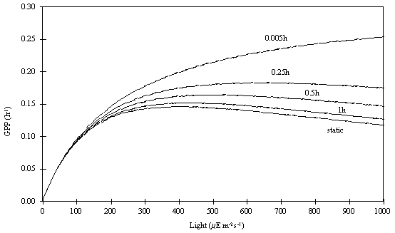
Fig. 1 -
Effect of exposure time to light on gross productivity calculated with the
static and the dynamic version of the Eilers and Peeters’ model (see text).
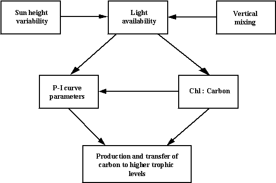
Fig. 2 -
Interdependence between the forcing functions and variables considered in the
present model.
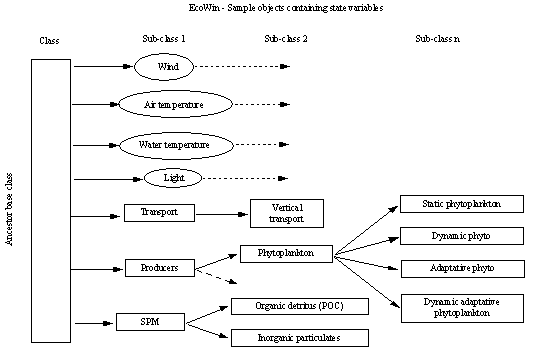
Fig. 3 -
Object structure of EcoWin.
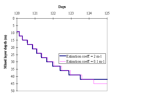
Fig. 4 -
Evolution of the mixed layer depth predicted by the model in the two case
studies - clear water and turbid water (see text).
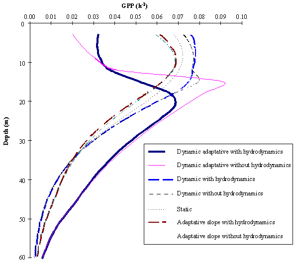
Fig. 5 -
Average gross productivity in carbon units during the five days of simulation,
between 0 and 60 m depth.
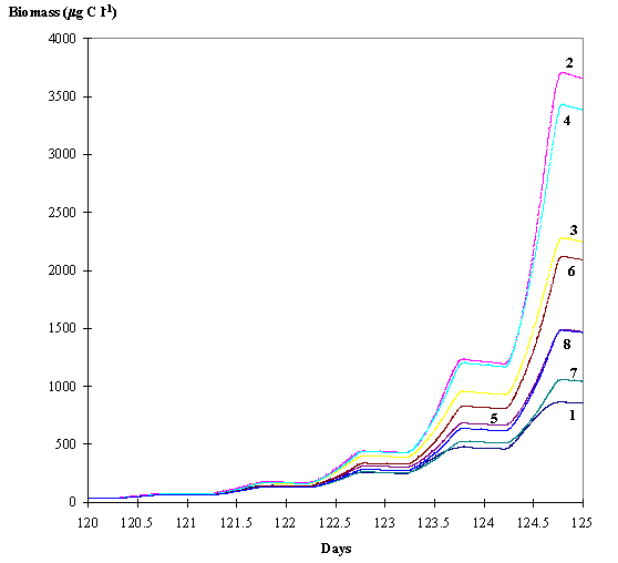
Fig. 6 -
Average phytoplankton biomass within the euphotic layer predicted by the eight
model simulations . 1 - Dynamic adaptative phytoplankton with hydrodynamics; 2
- Dynamic adaptative phytoplankton without hydrodynamics; 3 - Dynamic
phytoplankton with hydrodynamics; 4 - Dynamic phytoplankton without
hydrodynamics; 5 - Static phytoplankton with hydrodynamics; 6 - Static
phytoplankton without hydrodynamics; 7 - Adaptative phytoplankton with hydrodynamics;
8 - Adaptative phytoplankton without hydrodynamics (see text).
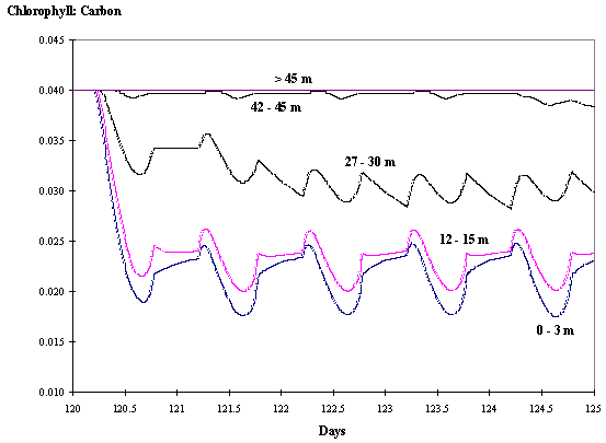
Fig. 7 -
Chlorophyll : Carbon ratio at various
depths as a function of time with hydrodynamics (see text).
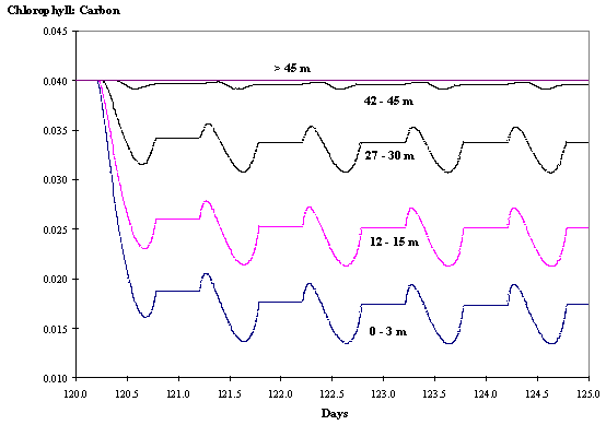
Fig. 8 -
Chlorophyll : Carbon ratio at various
depths as a function of time without hydrodynamics (see text).
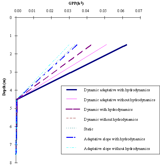
Fig. 9 -
Average gross productivity during the five days of simulation, between 0 and 9
m depth.
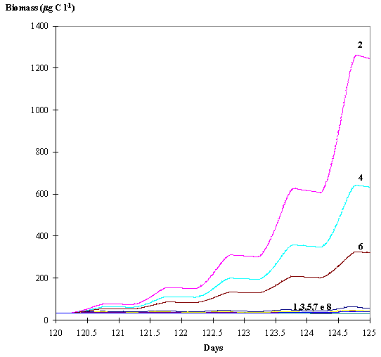
Fig. 10 -
Average phytoplankton biomass within the euphotic layer predicted by the eight
model simulations. 1 - Dynamic adaptative phytoplankton with hydrodynamics; 2 -
Dynamic adaptative phytoplankton without hydrodynamics; 3 - Dynamic
phytoplankton with hydrodynamics; 4 - Dynamic phytoplankton without
hydrodynamics; 5 - Static phytoplankton with hydrodynamics; 6 - Static
phytoplankton without hydrodynamics; 7 - Adaptative phytoplankton with
hydrodynamics; 8 - Adaptative phytoplankton without hydrodynamics (see text).
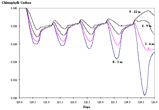
Fig. 11 -
Chlorophyll : Carbon ratio at various
depths as a function of time with hydrodynamics (see text).
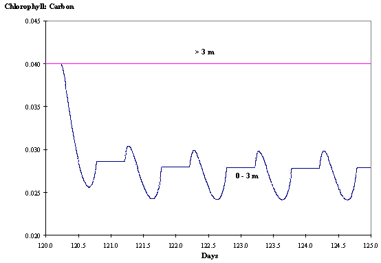
Fig. 12 -
Chlorophyll : Carbon ratio at various
depths as a function of time without hydrodynamics (see text).