A MODEL FOR THE SIMULATION OF MACROALGAL POPULATION
DYNAMICS AND PRODUCTIVITY
P. Duarte and J.G. Ferreira
Dept. Environmental Sciences &
Engineering, Faculty of Sciences and Technology
New University of Lisbon
2825 Monte de Caparica, Portugal
joao.imar@mail.telepac.pt
ABSTRACT
In this work a mathematical model to simulate the
population dynamics and productivity of macroalgae is described. The model
calculates the biomass variation of a population divided into size-classes.
Biomass variation in each class is estimated from the mass balance of carbon
fixation, carbon release and demographic processes such as mortality and frond
breakage. The transitions between the different classes are calculated in
biomass and density units as a function of algal growth. Growth is computed
from biomass variations using an allometric relationship between weight and
length. Gross and net primary productivity is calculated from biomass
production and losses over the period of simulation. The model allows the
simulation of different harvesting strategies of commercially important
species. The cutting size and harvesting period may be changed in order to
optimise the calculated yields.
In this study the model was used with the agarophyte Gelidium sesquipedale (Clem.) Born. et Thur.. This species was chosen
because of its economic importance as a the
main raw material for the agar industry. Net primary productivity
calculated with it and from biomass variations over a yearly period, gave
similar results. The results obtained suggest that biomass dynamics and
productivity are more sensitive to the water light extinction coefficient than
to the precision in biomass estimates, used as initial conditions for the
model. Model results also suggest that biomass losses due to respiration and
exudation are comparable to those resulting from mortality and frond breakage.
During winter, a significant part of the simulated population has a negative
net productivity. The importance of considering different parameters in the
productivity light relationships in order to account for their seasonal
variability is demonstrated with the model results.
The model was implemented following an object oriented
programming approach. The programming methodology allows a fast adaptation of
the model to other species without
major software development.
INTRODUCTION
Models to evaluate the population dynamics and
productivity of macroalgae are not common in the literature, in spite of the
importance of these algae in carbon fixation in coastal ecosystems. Models of
macroalgal populations may be divided into two groups:
i - Demographic models, that simulate the numerical
density of a population divided into size classes or different life history
phases (e.g. Ang , 1987, 1990; Chapman, 1993; Santos, 1993a);
ii - Models that simulate the biomass density
dynamics (e.g. Brinkhuis, 1977; Seip et al., 1979; Seip, 1980a e b; Ferreira
& Ramos, 1989; Duarte & Ferreira, 1993);
The first group is also known as "Leslie matrix
models" due to the influence of this author's work in their development
(Leslie, 1945, 1948). A revision on plant demographic models is given by
Caswell (1986). The general matrix model form, that can be adapted for age,
size or stage classified populations is, in matrix notation
![]() (1)
(1)
Where nt is a column vector with elements nt,1, nt,2... representing the number of
individuals in each class at time t
and nt+1 is another column
vector representing the number of individuals in each class at time t+1. A is the transition matrix
containing the probability transitions between the classes.
These
probabilities are a function of the growth, breakage, mortality and recruitment
rates of the different classes. Growth is the net result of physiological and
demographic time dependent processes leading to gains and losses of biomass.
Transition probabilities may be assessed by tagging macroalgal fronds of
different sizes and monitoring them during months or years, by measuring their
length and counting the survivors between sampling times. The transition rates
obtained are time-dependent due to various seasonal phenomena. This variability
complicates the application of these models to forecasting, unless the
transition probabilities are expressed as functions of the environmental
variables on which they depend. However, usually this is not the case. An
example of the application of this type of model to maximise harvest yields of
marine macroalgae is found in Ang (1987).
In
models of the second type, the population biomass is usually expressed as a
whole (e.g. frequently as a carbon pool) without discriminating between size or
life history phases. These models are often employed in primary productivity
calculations. The biomass variations are usually computed from the
physiological and demographic processes that are calculated as a function of
physical and chemical parameters. The general equation for macroalgae is
![]() (2)
(2)
Where,
B - Biomass, T - Time, P - Gross
productivity, R - Respiratory rate, F - Photorespiratory rate, E - Exudation rate, Q - Frond breakage rate, M -
Mortality.
During the last decades several mathematical
formulations of algal primary productivity (P)
as a function of light intensity have been developed (e.g. Steele, 1962; Jassby
& Platt, 1976; Platt el al. 1980;
Iwakuma & Yasuno, 1983, Eilers & Peeters, 1988). Equations that combine
the effects of several environmental variables such as light intensity,
temperature and nutrient concentrations can also be found (e.g. Keller, 1989).
These mathematical formulations were developed mainly for phytoplankton
although there seems to be no reason against their employment in macroalgal
productivity, since the underlying physiological phenomenon is the same. It has
been demonstrated that carbon fixation in marine macroalgae may also occur in
the absence of light (Kremer, 1981). In some Phaeophyceae the dark carbon
fixation may account for up to 50 % of the total carbon assimilated. In the
Chlorophyceae and Rhodophyceae the dark fixation is very low, corresponding to
approximately 3 % of the total.
It is generally accepted that respiration, like any
other biochemical reaction, is temperature dependent (Margalef, 1977) through
an Arrhenius function (Odum, 1983). Photorespiration and exudation are usually
expressed as constant rates or fractions of the gross productivity. The
demographic processes of frond breakage and mortality are very difficult to
simulate due to their high stochastic variability, but they may be estimated by
monitoring tagged fronds.
A third type of model may be defined by combining
types i) and ii) and simulating simultaneously biomass and numerical density of
pre-defined size-classes as a function of time. Instead of calculating the
transitions between classes using probability estimates, these transitions are
computed from the average individual growth of the classes, which is estimated
from allometric relationships based on changes of the average individual
weight. The changes of the average weight are calculated from the biomass
change (eq. 2) and the numerical density of each class.
The utilisation of size classes is crucial when
modelling a harvestable resource. When the objective is to attain a sustainable
yield, it is important to know the proportion of the harvestable and
non-harvestable classes and the rate at which the former recover from the
harvest (Usher, 1966). To develop a management strategy which takes into
account the variability of different environmental factors, it is important to
combine type i) and ii) models into the type iii) approach.
In the present work a model of this last type was
developed and applied to the species Gelidium
sesquipedale. This species is a clonal agarophyte red alga that grows
mainly in the subtidal by the continuous production of upright fronds from a
prostrate system of colourless axes (Dixon, 1973). Plants above 4-5 cm are
usually branched.
In recent years, studies were conducted by Santos
& Duarte (1991) and Santos (1993a, b, c, 1994) on the management,
population dynamics and ecology of this species off the west coast of Portugal.
Some of the conclusions arising from the works of this author are the
following:
1. The development of G. sesquipedale stands is favoured by high substrate slopes and low
sedimentation rates;
2. Frond breakage due to wave action is a very
important factor in the population dynamics of this species;
3. Growth is seasonal, occurring mainly during spring
and summer;
4. The intraspecific competition is kept at very low
levels due to high mortalities and frond breakages;
The productivity and respiration rates of G. sesquipedale were measured in field
conditions under different light intensity and temperature conditions (Duarte
& Ferreira, 1993). Studies conducted by Duarte & Ferreira (1995)
describe the functional dependency of G.
sesquipedale primary productivity on light intensity and temperature as
well as of respiration on temperature. Experimental evidence suggests that
these dependencies change with time as a result of seasonal adaptations. Winter
acclimated algae have lower photosynthetic efficiencies and higher respiratory
rates at ambient temperatures than summer acclimated ones. The conjunction of
these phenomena with lower photoperiods and light intensities may result in a
negative net productivity during winter.
METHODOLOGY
The methods used for model parameter estimation were
similar to those described in Duarte & Ferreira (1993) with the difference
that the functional relationship of productivity on light intensity and
temperature and of respiration on temperature were studied in the laboratory
under controlled conditions. The approach of combining biomass harvesting
methods, tagging experiments and short-term incubation productivity
measurements was the same as in the mentioned study. For details regarding
experimental procedures see Duarte & Ferreira (1995).
Sampling
As described earlier (Duarte & Ferreira, 1993),
sampling was carried subtidally (between 8 and 13 m depth) at Cape Espichel, a G. sesquipedale harvest area off the
west coast of Portugal (Fig. 1), over a 17 month period using scuba. Five 0.16
m2 quadrats were collected monthly by scraping the rock surface.
After cleaning of epiphytes, the dry weight biomass of G. sesquipedale fronds was determined.
(Fig.
1, near here)
Over the same sampling period 100-200 tagged G. sesquipedale fronds were monitored
monthly, in order to assess the mortality by the decline of tagged plants and
the breakage ratios by the reduction in frond size, by counting and measuring
the survivors between successive sampling campaigns. Data collection was
performed in the same area and with identical procedures as used earlier by
Santos (1993b), allowing a data analysis over a longer time period.
A fraction of the plants collected at each sampling
time were analysed in a Carlo Erba auto-analyser and their carbon, nitrogen and
phosphorus contents determined.
Net primary productivity
Daily and annual productivity estimates were obtained
for comparison with the model results. These estimates were computed from data
on biomass variation and on the loss and breakage rates of tagged fronds. The
population was divided in four size classes - <5, 5-10, 10-15 and >15 cm
- named classes 1, 2, 3 and 4. For each interval between two sampling periods
daily productivity was calculated with the equation
 (3)
(3)
![]()
NPP - Net primary productivity (g m-2 day-1);
B - Biomass (g m-2) ;
M - Losses through mortality (g m-2);
Q - Biomass removed by frond breakage (g m-2);
k - Size class;
n - total number of classes - 4;
t
- Number of days between
two consecutive samples.
Annual productivity was estimated by summation of the
products of daily estimates over the respective sampling periods during a year.
Mortality was calculated from the loss rates of tagged
fronds between two consecutive samples. It was assumed that the fraction of
biomass lost by mortality was equal to the fraction of individuals lost from
the population, since no relationship was found between mortality and plant
size. Tag loss was estimated by double tagging several thalli (Santos, 1993b).
Biomass loss through partial frond breakage was
calculated in two steps:
1) An empirical relationship between frond length and
daily breakage probability was obtained (Fig. 2);
2) An empirical relationship between frond length and
daily length reduction by breakage was also obtained (Fig. 3).
(Figs.
2 and 3, near here)
These relationships were calculated from data
collected by Santos (1993a) between August 1989 and September 1990 and by the
authors between September 1990 and October 1991. The first relationship was
used to compute the percentage of fronds that were broken daily between two
consecutive samples in each class. The second relationship was used to
calculate the average daily reduction in the length of the fronds that were
broken. A allometric relationship was used to compute the weight from the
length before and after breakage. The difference in both weights gives the
biomass lost by each frond. The product of this biomass by the breakage
probability and the density of each class gives the total biomass lost per day
per class.The total lost during the period t is given by the product of the daily biomass loss by
the number of days between two consecutive samples.
Modelling
Model
general structure and conceptualization
The main model equations are shown in Table 1. All
computations are carried out for each size-class. From the net gain or loss in
biomass and the number of individuals in each class the average individual
weight of the class is computed. From an allometric relationship (eq. 4) the
size is calculated. Growth is computed as the difference between the newly
calculated size and the previous size.
(Table
1, near here)
 (4)
(4)
(p < 0.001)
In the present case it is assumed that photosynthesis,
respiration and exudation are independent of plant size. However, frond
breakage is computed as a function of average class length as in the primary
productivity computations (see above). Competition with other species is not
considered. The comparison of the growth rates of tagged fronds with and
without epiphytic algae did not show any significant differences (Duarte &
Ferreira, 1993). Intraspecific competition seems to be reduced by the
occurrence of storms and harvest, leading to major biomass losses (Santos,
1993a). Mortality is calculated as a constant fraction of the biomass and was
obtained from the loss rate of tagged fronds. It is assumed that the population
is in steady-state concerning the numerical density of the individuals:
Therefore, dead fronds are replaced by class 1 recruits. Frond breakage is
computed as described above. Photorespiration was not considered due to the
absence of data on G. sesquipedale.
Parameter
fitting
Gross productivity is expressed as a function of light
intensity and temperature by a model described previously (Duarte, in press). Different parameters were
used according to season or depth. These parameters were obtained by studying
the relationship of productivity with light intensity and temperature on algae
that were previously acclimated to different conditions. Four types of
acclimation were employed, two simulating winter conditions and two different
depths - approximately 9 and 13 m - and two simulating summer conditions and
the same depths. Experimental evidence suggests that the model parameters are
dependent on the recent history of the plants (Duarte & Ferreira, 1995). The equations for productivity
calculation and respective parameters are shown in Table 2. At every time step
the equation that was obtained with algae acclimated to conditions closest to
the simulated ones was chosen. Equations obtained with algae from the winter
acclimation were employed for winter and autumn simulations. Equations obtained
with algae from the summer acclimation were employed for summer and spring
simulations. Interpolation between the results obtained with different
equations was carried out whenever the simulated conditions were within the
range of the acclimation depths. A similar approach was used for respiration
although this process was expressed solely as a function of temperature and
season (Table 2). The conversion of productivity and respiration expressed in
carbon units to biomass units was based on the carbon content of the studied
species.
(Table
2, near here)
Exudation rate was also measured during the above
mentioned experiments. Slightly different values were obtained with algae from
the different acclimations. It was not possible to express exudation as a
function of any environmental variable so it was computed as a rate that
changed only with season or depth. The appropriate value was chosen following
the same criteria used in the choice of equations for productivity calculation.
Size
class structure and transitions
The usage of any kind of categories in mathematical
modelling, such as size classes or compartments, usually implies that all
individuals within a size class are assumed to be of the same size. In the
Leslie matrix models the transitions between the classes occur in a progressive
way, since the transition probabilities are usually less than one. The usual
exceptions to this rule are the transitions to class 1 because each individual
belonging to the larger size classes may produce more than one recruit.
In the present model the growth in each size class is
computed from the net gains in weight. If it is assumed that all individuals
are of the same size, the transition from one class to another occurs at the
same time for all individuals of the departure class. This discrete type of
transition may be acceptable when the size classes cover a very narrow range of
sizes, but loses realism when the size classes are wider. Discrete transitions
can lead to unreliable results when one or more size classes are emptied of
individuals and the size distribution of the population becomes discontinuous,
since in natural conditions this does not usually happen. Such transitions also
tend to increase model instability. A possible solution to this problem is the
usage of a statistical distribution of size within each class. In this case the
growth of the individuals can be used to estimate their transition
probabilities to a neighbouring size class.
In the present work the size distribution of
individuals within each class was assumed to be gaussian. This assumption is a
simplification, as well as the usual assumption of homogeneity. Its test
against field data gave controversial results. In some cases the assumption
seemed to be a good approximation whereas in other cases it was not validated.
In fact, in a algal population where age-classes are not possible to define (as
in the present case) there is no reason for this assumption to be always valid.
But any assumption regarding intra-class structure will suffer from some
disadvantages, specially when size-classes are considered.
To define a normal distribution two parameters are
needed; the mean and the standard deviation. In the present case the mean is
the current size of each class computed with the model at every time step. The
standard deviation is unknown, but a value can be obtained to force the
distribution to "stay" within the class limits. The values 2.5 were assumed to be the "limits" of the
normal distribution. These values include more than 99% of the area under the
standard normal curve, and were used as the standardised limits for the size
classes. The standard deviation is computed as the minimum of the following
equations:
![]() (5)
(5)
![]() (6)
(6)
The transitions of individuals may occur both to
larger and smaller classes. In the first case, the transition will tend to
decrease the average size of the destination class, whereas in the second case
the opposite is true. The transition to smaller classes may occur through the
breakage of the fronds, being more important when net productivity is negative.
By knowing the mean size, its standard deviation and growth it is possible to
calculate a critical standardised value above which the individuals should be
transferred to another class
![]() (7)
(7)
The class limit to consider is the upper one if growth
is positive and the lower one if growth is negative.
In Fig. 4 the effect of growth on the shape of the
distribution is shown. The distribution shifts to the right and becomes
narrower. All individuals above the critical limit are transferred to the
neighbouring size class. The area of the curve to the right of the critical
limit is calculated by integration. In the present work the formula of Hastings
was used. It is important to remark that during the mentioned transitions
biomass is conserved.
(Fig.
4, near here)
A total of 12 classes was used in model calculations:
<5, 5-6, 6-7, 7-8, 8-9, 9-10, 10-11, 11-12, 12-13, 13-14 and >15 cm.
However, for output only 4 classes were considered: <5, 5-10, 10-15 and
>15 cm. Only the upper limit is included in each of the classes considered.
The greater the number of classes used in model calculations the more
reasonable is the assumption of homogeneity within the classes.
To preserve model stability, asymptotic biomass values
were assumed for each class. These values were chosen from the maximal biomass
observed in Cape Espichel (over 500 g (DW) m-2). When the biomass of
a class is greater than its asymptotic value, the excess biomass and
corresponding individuals are transferred randomly to the smaller classes or to
the next class, simulating frond breakage or growth. If the excess occurs in
class 1 then biomass is transferred to class 2. If the excess occurs in the
last class, all biomass is transferred to smaller classes.
Model forcing functions
Daily water temperatures and global surface radiation
obtained in two meteorological stations located near the study area were used
as forcing functions for the model. Tidal height was simulated as described in
Ferreira & Ramos (1989). Underwater light intensity was computed as described
in Duarte & Ferreira (1993).
Nutrients were not used as forcing functions to the
model. The capacity that some macroalgae have for luxury consumption makes the
description of nutrient limitation more complicated. This capacity has been
demonstrated for Gelidium species by
Fredriksen & Rueness (1989). In the present case, dissolved nutrient data
exists, but the available results do not allow the description of nutrient
limitation.
Software development
Implementation of the model was carried out using
object-oriented programming integrated in a existing model structure called
EcoWin (Ferreira, 1995). An object named Gelididium
sesquipedale was developed containing all attributes (variables) and
methods (functions) used in the model calculations. A "man" object
was also developed to simulate the harvest of the studied population. By
coupling/uncoupling this object the impact of harvest on the studied population
can be assessed. Different harvesting strategies can be simulated by simply
changing the initialisation of some model conditions.
RESULTS AND DISCUSSION
G. sesquipedale population dynamics and productivity
Frond breakage probability and frond length reduction
by breakage increase with frond initial size (Figs 2 and 3). The larger fronds break easier than the
smaller ones and the reduction in size is greater in the former than in the
latter. These results can be explained by the fact that the larger fronds
suffer greater drag induced by waves and currents (Koehl, 1986; Denny, 1988).
In fact, frond breakage (Fig. 5) seems to be more related to frond size than to
any seasonal factors, since the largest breaking ratios were observed in summer
months when average frond size is higher (see above) and wave stress is lower.
Wave height rarely exceeds 2 m during summer, whilst in winter values above 3
and 4 m are frequent in the west coast of Portugal.
(Fig.
5, near here)
In Fig. 6 frond mortality is shown, including the
results obtained by Santos (1993a). The correlation between frond mortality and
frond length is not significant (p > 0.05). Mortality does not seem to
follow a distinct pattern throughout the year. The highest values were observed
between August and September 1990 and between June and July 1991. The first
maximum could be related to harvest in the study area (Santos, 1993a). The
second maximum could be related to a worsening of sea conditions.
(Fig.
6, near here)
The biomass density dynamics of the studied species is
shown in Fig. 7, together with the model results. Maximal values were observed
during summer whilst minimal values occurred in winter. Similar results were
obtained by Santos (1993a) in the same study area and by Juanes & Borja
(1991) in the North of Spain.
(Fig.
7, near here)
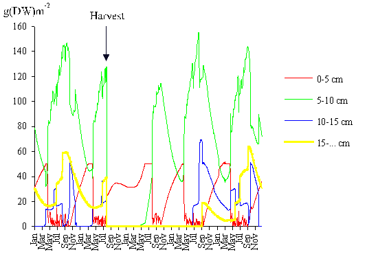
The biomass dynamics of the four classes considered is
shown in Fig. 8. The algae belonging to the intermediate sizes (classes 2 and
3) are dominant in terms of biomass. The larger fronds tend to increase their
importance from spring to summer. This is also confirmed by Santos (1993a).
During autumn and winter the biomass decreases due to mechanical stresses and
metabolic losses affects all classes. However, the smaller classes are less
affected because they receive a biomass input from the larger classes due to
the breakage of the larger fronds.
(Fig.
8, near here)
Net primary productivity calculated by the method
described in this work is shown in Table 3. The losses through mortality and
frond breakage were larger than the net productivity. The reason for this
result is that during the period used for productivity computation (May 1990 -
May 1991) a net loss of biomass occurred. The average daily net primary
productivity between sampling periods is shown in Fig. 9. The estimated values
range between -2 and approximately 6 g (DW) m-2 day-1.
Negative values occur mainly in autumn and winter months.
(Fig.
9 and Table 3, near here)
Model results
Standard
simulation
Further parameter optimisation for the standard
simulation was carried out after model calibration. The water extinction
coefficient was the only parameter used in this final optimisation. Its value
was set equal to 0.22, well within the range of the observed values (0.26 0.09) in the study area for a period of over a year.
Model results were integrated over a depth range from 8 to 10 m with respect to
the tidal datum, including the range of depths at which biomass sampling and
tagging experiments took place.
In Fig. 7 the model biomass predictions and the
observed values for the period between May 1990 and October 1991 are shown.
Almost all model results are within the confidence limits of the observed
values. The correlation between the measured and the predicted values is 0.74
(p < 0.05).
In Table 3 the annual net primary productivity
predicted by the model can be compared to the value calculated by the method
based on biomass differences, mortality and breakage ratios. The model
prediction is only 15 % higher than the values estimated with this method.
In Fig. 10 the model biomass prediction is shown for a
period of about five years, showing that after the second year of simulation
the model remains stable. In Fig. 11 the model biomass prediction for each of
the four classes is also shown for the same time interval. After the second
year of simulation the population structure follows a pattern similar to that
observed in Fig. 8, except that the biomass density of classes 1 and 4 is
slightly higher than expected from field results.
(Fig.
11, near here)
In Fig. 12 the daily gross and net productivity
predicted by the model are shown. Net primary productivity values obtained with
the model are well within those estimated by the method described in this work.
In autumn and winter net primary productivity is predominantly negative. These
results can be explained by the low light intensities and temperatures during
those seasons (Fig. 13) and were predicted earlier by the authors from
laboratory data (Duarte & Ferreira, 1995). Considering that most of the G. sesquipedale stands on the west coast
of Portugal are found at greater depths than those simulated (8 - 10 m), the
negative net productivity during these seasons is probably more a rule than an
exception.
(Fig.
12 and 13, near here)
The model results reported in Table 3 suggest that the
greatest part of the biomass loss is attributable to mortality and frond
breakage. The losses due to respiration and exudation are of the same order of
magnitude. Since mortality and frond breakage are part of the net primary
productivity, the negative values of this parameter are explained solely by the
respiration and exudation losses. As suggested earlier (Duarte & Ferreira,
1995), the lower photosynthetic efficiencies of the winter acclimated plants,
together with the lower light intensities and shorter photoperiods occurring in
winter and autumn, explain the negative net productivity.
Sensitivity
analysis
The sensitivity of the model was tested against some
of the model initial conditions, forcing functions and parameters.
Sensitivity to the initial conditions
Concerning the initial conditions, the model
sensitivity to the initial biomass levels was investigated, in order to
evaluate the importance of the usually low precision of the biomass estimates
on model predictions. As initial biomass input to the model both the upper and
the lower confidence limits (at the 95 % confidence level) of the mean biomass
observed in May 1990 (161.4 and 71.3 g (DW) m-2, respectively) were
tested. This corresponds to a change of 39 % in relation to the average biomass - 116.3 g (DW)
m-2. The larger biomass led to a net productivity prediction 38 %
higher than under the standard simulation. The lower biomass led to a net productivity
37 % lower than under the standard simulation (Table 4).
Sensitivity to the model forcing functions
Concerning the model forcing functions, the
sensitivity of the model to changes in the water light extinction coefficient
and to temperature was tested. A 10% increase in the extinction coefficient led
to a annual net productivity prediction of 104.0 g m-2 year-1,
which is 45 % lower than the result obtained under the standard simulation (Table
4). As before, during autumn and winter net primary productivity is
predominantly negative (not shown). A 10% decrease in the extinction
coefficient was also tested. In this case a 61 % increase of the predicted
primary productivity in relation to the standard simulation was obtained (Table
4).
From the above results it follows that the model is
more sensitive to the light extinction coefficient than to the initial biomass
conditions. The greater sensitivity of the net as compared to the gross primary
productivity to the extinction coefficient are explained by the lower values of
the latter. If gross productivity is affected by a change, the corresponding
change in net productivity (which is the difference between gross productivity
and the loss processes of respiration and exudation) will tend to be higher
unless there is a similar change in respiration and exudation.
The sensitivity to temperature was investigated by
assuming an average Summer temperature equal to the average Winter-Spring
values (15 ºC). The predicted reduction in productivity (Table 4) demonstrates
the potential for temperature limitation, since values close to 15 ºC can
sometimes be observed during Summer (Fig. 13). In this case net productivity is
less affected than gross productivity because the reduction in the latter
during Summer is accompanied by a reduction in the respiration rates due to the
lower temperatures.
Sensitivity to the model parameters
The sensitivity to mortality and breakage ratios were
investigated by changing the default values to 10 %. From the results shown in Table 4 it is clear
that the model is more sensitive to changes in mortality than to changes in the
breakage ratio which in fact are almost irrelevant in the model output. The
model sensitivity to changes in mortality is also low. Since both mortality and
the breakage ratios are very difficult to estimate and subject to many errors
the low model sensitivity to them is an important result. The higher
sensitivity of gross rather than net productivity to changes in mortality is
explained by the fact that the changes in gross productivity at the population
level reflected by the changes in the biomass standing stock resultant from
different mortalities, are accompanied by changes in the population respiration
rates, which tend to compensate for changes in net productivity.
The sensitivity of the model to the usage of only one
set of parameters in the productivity equation was also investigated (shown in
eq. 8). The parameters were estimated by analysing together the four data sets
used in the parameter estimation of equations 12 to 15 (see Duarte &
Ferreira, 1995). As can be seen in Table 4 the predicted annual productivity
estimates are much lower (-14.1 and -17.9 % for annual gross and net
productivity, respectively) than those obtained under the standard simulation.
The nonlinearities between productivity and the forcing functions light and
temperature may explain this result which highlights the importance of
considering seasonal adaptation on primary productivity simulation.
 (8)
(8)
A similar approach was followed concerning respiration
(eq. 9). In this case the differences relative to the standard simulation are
smaller (Table 4). This may be partly explained by the fact that the annual
losses by respiration are much lower than the annual net productivity (Table
3).
![]() (9)
(9)
(Table
4, near here)
Harvest simulation
Harvest usually takes place from the end of July to
the end of the year. In the following simulations it was assumed that the
plants were cut instead of plucked from the rocks, since the disadvantages of
this harvesting technique have already been discussed and demonstrated (Salinas et al., 1976; Santelices, 1988;
Santos, 1993c). There are already cutting devices operated from boats that
allow the cutting height to be chosen and do not decrease the plant density
(Santos, 1993c). It was assumed that cutting occurred only once in a
hypothetical 1 m2 area. The recovery of the population was then
followed. The initial conditions were those of the standard simulation after
allowing the model to reach stability.
In the first of these harvest simulations a cutting
height of 3 cm was assumed, with harvest taking place at the end of July,
leaving all harvested plants with a length of 3 cm after cutting. In Fig. 14
the predicted results are shown. After harvest, the remaining biomass was
approximately 13 % of the initial value. Three years later, the recovery of the
population was complete. The total harvested biomass was 167 g (DW) m-2.
All individuals entered into class 1 after cutting. The recruitment to class 2
occurred in the first year after the harvest, whilst the recruitment to classes
3 and 4 occurred only in the second year (Fig. 14). Since the lower dimensional
limit of class 4 is 15 cm, it follows that the algae that recruited to this
class grew approximately 6 cm year-1 after harvest. The growth rates
referred by Santos (1994) point to an annual maximum of 8 - 9 cm. However,
these results were obtained by considering only the tagged algae that grew
between two measurements, so they correspond to a potential maximal growth rate
that is hardly ever attained.
(Fig.
14, near here)
Further simulations were carried out assuming cutting
heights of 5, 7 and 9 cm. The results obtained are synthesised in Table 5,
where the average annual yield is plotted against the time for the population
to recover after cutting. It was assumed that cutting is not repeated until
full recovery of the population. A cutting height smaller then 7 cm may lead to
a regrowth period of two years or more. By keeping the cutting height around 7
cm it is possible to harvest every year and to obtain an average yield larger
then cutting to a lesser height every two or three years. These results
demonstrate the potential usefulness of the model and suggest some interesting
options to increase harvest yield.
(Table
5, near here)
The results obtained confirm that during autumn and
winter the primary productivity of an important part of the G. sesquipedale stands is negative.
During these periods major biomass losses occur because of storms and metabolic
losses. This natural "harvest" may be anticipated by an industrial harvest,
that may be kept at a sustainable yield by appropriately choosing the cutting
heights and harvesting frequency.
CONCLUSIONS
The main objective of this model was to simulate
simultaneously the frond individual weight/size, the biomass and density changes
of an algal population divided in size classes. The simulation of the frond
size is important when the population is to be harvested and the optimal
cutting height is to be defined. Besides that, only by simulating size is it
possible to describe some demographic aspects and control some model results in
terms of their quality. For example, it is important to calibrate the model in
order that the size of the plants does not exceed a maximal value, determined
from field data. When this value is reached the breakage ratio should be
reformulated in order to avoid any further growth.
The usage of size classes has important implications
in model calibration and validation, since the distribution of biomass among
the classes follows certain patterns that must be taken into account during the
modelling process. If classes are not considered and biomasses treated as a
single class the predicted values are much higher than when classes are
considered and asymptotic biomass values (see Method's section) are defined for
each class. The rationale behind the use of these asymptotic values is related
to those processes that are either not explicitly or poorly simulated by the
model, such as space limitation and frond breakage ratios.
The assumption that the distribution of sizes within
the classes follows the normal distribution and the usage of the algorithm
described previously, allowed the simulation of the biomass transfer between
classes in a quasi-continuous way. It is likely that the methods described here
concerning between-class transfer can be employed in the simulation of other
plant and animal populations. The assumption of normality is debatable, but the
usual assumption of size/weight homogeneity within the classes is also arguable
and leads to unreliable delays in the between-class transfer. These problems
can be partially solved only by considering a very large number of classes
which are reflected in more computing time. In the case of animal or plant
populations in which cohorts are easy to define, the assumption of normality in
size/weight distributions within the classes is less questionable since it is
clear that these distributions are close to normal.
Further improvements of the present model include the
dynamic description of photosynthesis in a way similar to that discussed by
Pahl-Wostl & Imboden (1990). The equations used in the present work do not
take into account the developing time of photoinhibition. This may be done by
describing the first parameter (responsible for the photoinhibited behaviour)
of the denominator of equations 14-17 as a function of the time the plants are
exposed to a light level above the optimum. The authors' results (unpublished)
suggest that under certain conditions the predicted primary productivity may be
much higher than expected by considering this time dependency. However, the
available data does not allow an accurate estimation of its importance for the
studied species.
Another important field of research is the seasonal
adaptation of the photosynthetic and respiratory responses to light and
temperature. The usage of different equations according to time of the year or
depth as in the present work, is far from optimal. However, it was the only
available way to include some of the variability for these responses.
It is also important to consider the time variability
of the allometric relationships used to calculate growth from biomass changes
and vice-versa. These relationships are expected to change over time because,
among other things, of the endogenous annual cycles (Lüning, 1993) demonstrated
for some algal species. The growth in weight may not always coincide with the
growth in length.
The usage of an object oriented programming approach
allows the fast development of descendants to any general object inheriting
their attributes and methods (Silvert, 1993; Ferreira, 1995). In the present
case descendants to the G. sesquipedale
object may be developed as more information becomes available concerning any of
the topics just discussed. The programming work would consist only of adding
the new functions, or overriding the old ones. The extension of this model to
other species is likewise straightforward.
Acknowledgements
This work was supported by JNICT (PhD grant Nº154 -
IG) and INETI. The authors wish to thank C. Peneda for support of this
research, and L. Saldanha, L. Fonseca and O. Luis (LMG-IMAR) and F. Duarte
(INETI), for making available laboratory facilities. The authors also thank R.
Santos for making available part of his data and A. Afonso for his help on
statistics.
REFERENCES
Ang, P.O. Jr, 1987. Use
of projection matrix models in the assessment of harvesting strategies for Sargassum. Hydrobiologia, 151/152:
335-339.
Ang, P.O. Jr and De
Wreede, R.E., 1990. Matrix models for algal life history stages. Mar. Ecol.
Prog. Ser., 59: 171-181.
Brinkhuis, B.H., Tempel,
N.R. and Jones, R.F., 1976. Photosynthesis and respiration of exposed
salt-marsh fucoids. Marine Biology, 34: 349 - 359 .
Caswell, H., 1986. Life
cycle models for plants. In: Lectures
on mathematics in the life sciences, Vol. 18, pp. 171-223. Ed. by the American
Mathematical Society.
Chapman, A.R.O., 1993.
'Hard' data for matrix modelling of Laminaria
digitata (Laminariales, Phaeophyta)
populations. Hydrobiologia, 260/261: 263-267.
Dixon, P.S., 1973. Biology of the Rhodophyta. Oliver
& Boyd, Edinburgh.
Denny, M.W., 1988.
Biology and the mechanics of the wave-swept environment. Princeton University
Press, Princeton.
Duarte, P., 1995. A
mechanistic model of the effects of light and temperature on algal primary
productivity. Ecol. Modelling, 82: 151-160.
Duarte, P., and
Ferreira, J.G., 1993. A methodology for parameter estimation in seaweed
productivity modelling. Hydrobiologia, 260/261: 183-189.
Duarte, P. and Ferreira,
J.G., 1995. Seasonal adaptation and short-term metabolic responses of Gelidium esquipedale to varying light
and temperature. Mar. Ecol. Prog. Ser, 121: 289-300.
Eilers, P.H.C. and
Peeters, J.C.H., 1988. A model for the relationship between light intensity and the rate of photosynthesis in
phytoplankton. Ecol. Modelling, 42: 199 - 215 .
Ferreira, J.G. and
Ramos, L., 1989. A model for the estimation of annual production rates of
macrophyte algae. Aquatic Botany, 33: 53-70.
Ferreira, J.G., 1995.
ECOWIN - An object-oriented ecological model for aquatic ecosystems. Ecol.
Modelling, 79: 21-34.
Fredriksen, S. and
Rueness, J., 1989. Culture studies of Gelidium
latifolium (Grev.) Born et Thur.
(Rhodophyta) from Norway.Growth and nitrogen storage in response to varying
photon flux density, temperature and nitrogen availability. Botanica Marina,
32: 539 - 546.
Iwakuma, T. and Yasuno,
M., 1983. A comparison of several mathematical equations describing
photosynthesis-light curve for natural phytoplankton populations. Arch.
Hydrobiol., 97: 208-226.
Jassby, A.D. and Platt,
T., 1976. Mathematical formulation of the relationship between photosynthesis
and light for phytoplankton. Limnol. Oceanogr., 21: 540-547.
Keller, A.A., 1989.
Modeling the effects of temperature, light, and nutrients on primary
productivity: An empirical and a mechanistic approach compared. Limnol.
Oceanogr., 34: 82-95.
Koehl, M.A.R., 1986.
Seaweeds in moving water: form and mechanical function. In: Givnish, T.J. (ed.)
On the economy of plant form and function, Cambridge University Press,
Cambridge, pp. 603-634.
Kremer, B.P., 1981.
Aspects of carbon metabolism in marine macroalgae. Oceanogr. Mar. Biol. Ann.
Rev., 19: 41-94.
Leslie, P.H., 1945. On
the use of matrices in certain population mathematics. Biometrica, 33: 183-212.
Leslie, P.H., 1945. Some
further notes on the use of matrices in population mathematics. Biometrica, 35:
213-245.
Lüning, K., 1993.
Environmental and internal control of seasonal growth in seaweeds.
Hydrobiologia, 260/261: 1-14.
Margalef, R., 1977. Ecologia. Omega, Barcelona.
Odum, H.T., 1983.
Systems ecology: An introduction. John Wiley & Sons, Inc., Toronto.
Pahl-Wostl, C and
Imboden, DM, 1990. DYPHORA - a dynamic model for the rate of photosynthesis of
algae. J. Plankton Res., 12: 1207-1221.
Platt, T., Gallegos,
C.L. and Harrison, W.G., 1980. Photoinhibition of photosynthesis in natural
assemblages of marine phytoplankton. J. Mar. Res., 38: 687-701.
Salinas, J.M., Ramirez,
B.R. and Olivet, R.G., 1976. Biometría en Gelidium
sesquipedale (Rhodophyta). Bol. Inst. esp. Oceano., 225: 127-166.
Santelices, B., 1988.
Synopsis of biological data on the seaweed genera Gelidium and Pterocladia
(Rhodophyta). FAO Fisheries Synopsis, 145.
Santos, R. and Duarte,
P., 1991. Marine plant harvest in Portugal. Journal of Applied Phycology, 3: 11-18.
Santos, R., 1993a.
Plucking or cutting Gelidium sesquipedale?
A demographic simulation of harvest impact using a population projection matrix
model. Hydrobiologia, 260/261: 269-276 .
Santos, R., 1993b.
Population biology of the commercial seaweed, Gelidium sesquipedale: Biological input for resource management.
PhD Thesis, Dalhouise University, Halifax, Nova Scotia, Canada.
Santos, R. 1993c. A multivariate study of biotic and
abiotic relationships in a subtidal algal stand. Mar. Ecol. Prog. Ser., 94:
181-190.
Santos, R., 1994. Frond
dynamics of the commercial seaweed Gelidium
sesquipedale: effects of size and frond history. Mar. Ecol. Prog. Ser.,
107: 295-305.
Seip, K.L., Lunde, G.,
Melsom, S., Mehlum, E., Melhuus, A. and Seip, H.M., 1979. A mathematical model
for the distribution and abundance of benthic algae in a norwegian fjord. Ecol.
Modelling, 6: 133-166.
Seip, K.L., 1980a. A
computational model for growth and harvesting of the marine algae Ascophyllum nodosum. Ecol. Modelling, 8: 189-199.
Seip, K.L., 1980b. A
mathematical model of competition and colonisation in a community of marine
benthic algae. Ecol. Modelling, 10: 77-104.
Silvert, W., 1993. Object-oriented ecosystem
modelling. Ecol. Modelling, 68: 91-118.
Sokal, R.R. and Rohlf,
F.J., 1981. Biometry. The principles and practice of statistics in biological
research. W.H. Freeman & Co, San Francisco.
Steele, J.H., 1962.
Environmental control of photosynthesis in the sea. Limnol. Oceanogr., 7: 137 -
150.
Usher, M.B., 1966. A
matrix approach to the management of renewable resources, with special
reference to selection forests. J. Appl. Ecol., 3: 355-367.
Wiegert, R.G. and Evans,
F.C., 1964. Primary production and disappearance of dead vegetation on an oil
field in south-eastern Michigan. Ecology, 45: 49-63.
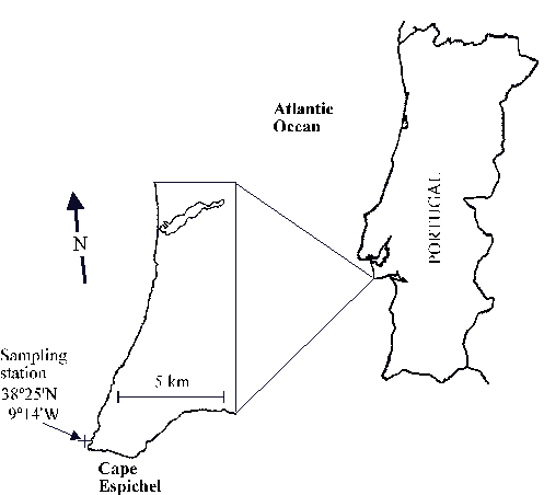
Fig. 1 - Study
area.
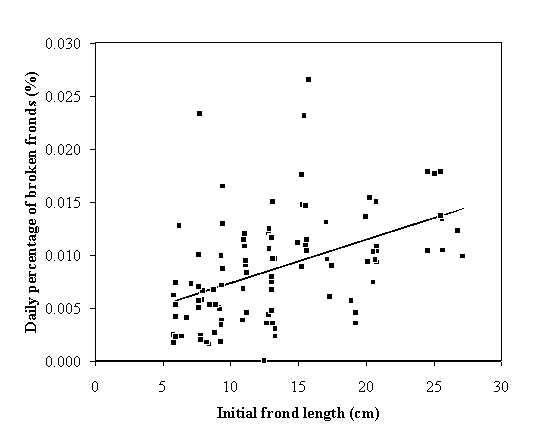
Fig. 2 - Average
daily percentage of broken fronds versus initial frond length. The regression
line (![]() ) is significant (p < 0.05).
) is significant (p < 0.05).
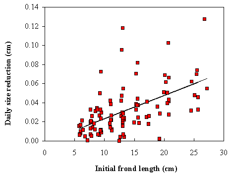
Fig. 3 - Size reduction versus initial frond length.
The regression line (![]() ) is significant (p < 0.001).
) is significant (p < 0.001).
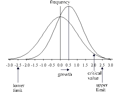
Fig. 4 - The
effect of growth on the shape of the size distribution of individuals within
the classes calculated by the model. The curve shifts to the right after growth
is computed. The area to the right of the critical value corresponds to the
transition probability (see text).
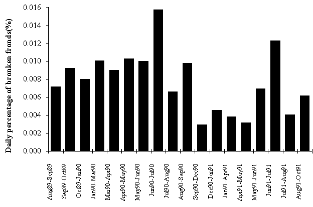
Fig. 5 - Frond daily breakage (% of tagged fronds).
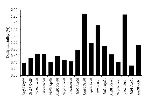
Fig. 6 - Daily
mortality (% of tagged fronds).
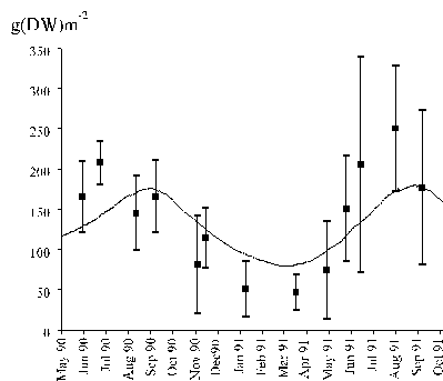
Fig. 7 - Biomass
density dynamics. Model results of the standard simulation (line) and observed
values (squares). The vertical bars are 95% confidence limits.
g(DW)m-2
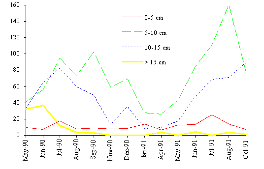
Fig. 8 - Biomass
density dynamics of the four classes considered.
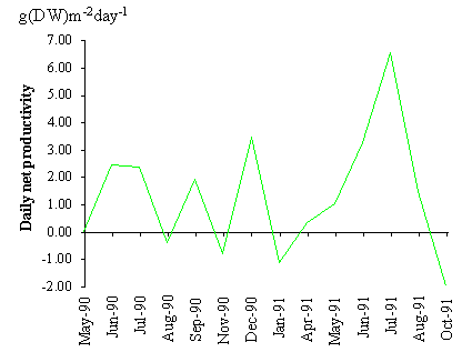
Fig. 9 - Daily
net productivity estimated by the method described in this work, from biomass
changes and losses due to mortality and breakage.
g(DW)m-2
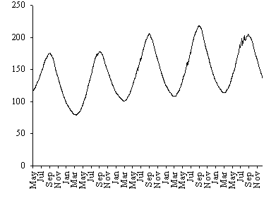
Fig. 10 -
Standard simulation. Biomass density predicted by the model.
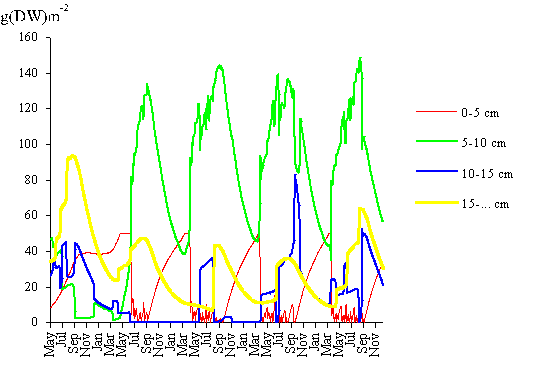
Fig. 11 - Standard simulation. Biomass density
variation of the four classes considered predicted by the model (see text).
g(DW)m-2
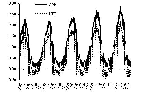
Fig. 12 - Standard simulation. Gross and net daily primary
productivity (GPP and NPP, respectively) predicted by the model.
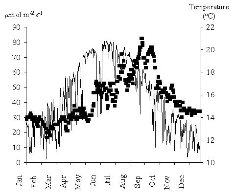
Fig. 13 - Daily average light intensity
(line) at 9 m depth (reported to tidal datum) and temperature (squares). The
light values were computed from available time series and assuming a water
light extinction coefficient of 0.22.
Fig. 14 -
Biomass density variation of the four classes considered predicted by
the model, before and after cutting the population to a height of 3 cm at the
end of July. All other conditions as in the standard simulation (see text).
Table 1 - Main
model equations.
|
|
(10) |
||
|
|
(11) |
||
|
|
(12) |
||
|
|
(13) |
||
|
B - Biomass (g m-2) z e z0-
Integration depths (m) T*= tf -
ti- Model timestep P' - Gross productivity(g C g-1 h-1)** R' - Respiration rate (g C g-1 h-1)*** P - Gross productivity (g m-2 T*-1) |
R -Respiration rate (g m-2 T*-1) E' - Exudation rate(g g-1 h-1) E - Exudation rate (g m-2 T*-1) Q - Frond breakage rate (g m-2 T*-1) M - Mortality (g m-2 T*-1) y - Conversion factor between carbon and dry
weight |
|
|
|
* 0.2 days. ** Computed as
a function of light intensity and temperature. *** Computed as
a function of temperature. |
|
||
Table 2 -
Equations for gross productivity and respiration; P' - Gross productivity (g C g-1 h-1), R' - Respiration rate (g C g-1 h-1***),
I - light intensity (mol photons m-2 s-1), t (ºC) (see text).
|
Acclimation |
Equations |
|
Winter 13 m
depth |
|
|
Winter 9 m
depth |
|
|
Summer 13 m
depth |
|
|
Summer 9 m
depth |
|
|
Winter |
|
|
Summer |
|
Table 3 - Annual productivity and biomass loss
estimates obtained by the method described in this work and by the model. GPP
and NPP - Gross and net primary productivity, respectively; POM - Losses
through particulate organic matter from frond mortality and frond breakage; DOM
- Losses through dissolved organic matter (exudation) and R - Respiration. All
values in g (DW) m-2year-1.
|
|
GPP |
NPP |
GPP/ Biomass |
POM |
DOM |
R |
|
Biomass differences and biomass removal estimates |
|
162.5 |
|
205.2 |
|
|
|
Model results |
339.3 |
187.7 |
2.9 |
210.0 |
51.1 |
100.6 |
Table 4 - Sensitivity analysis results (see text).
|
|
GPP |
NPP |
|
|
||
|
|
Calculated value (gDWm-2year-1) |
Relative change (%) |
Calculated value (gDWm-2year-1) |
Relative change (%) |
|
|
|
Standard simulation |
339.1 |
- |
187.5 |
- |
|
|
|
10% Increase in the initial biomass |
456.6 |
+34.7 |
257.8 |
+37.5 |
|
|
|
10% Decrease in the initial biomass |
214.0 |
-36.9 |
119.1 |
-36.5 |
|
|
|
10% Increase in the ext. coef. |
221.1 |
-34.8 |
104.0 |
-44.5 |
|
|
|
10% Decrease in the ext.coef. |
481.7 |
+42.1 |
301.6 |
+60.9 |
|
|
|
Using in Summer the average Winter-Spring temperature |
297.8 |
-12.2 |
160.6 |
-14.3 |
|
|
|
10% Increase in mortality |
329.8 |
-2.7 |
185.6 |
-1.0 |
|
|
|
10% Decrease in mortality |
367.5 |
+8.4 |
202.4 |
+7.9 |
|
|
|
10% Increase in frond breakage |
338.9 |
-0.1 |
187.4 |
-0.1 |
|
|
|
10% Decrease in frond breakage |
339.2 |
0.0 |
187.6 |
+0.1 |
|
|
|
Only one set of parameters in the prod. eq. |
291.4 |
-14.1 |
154.0 |
-17.9 |
|
|
|
Only one set of parameters in the resp. eq. |
338.3 |
-0.2 |
180.2 |
-3.9 |
|
|
Table 5 - Mean annual yield as a
function of regrowth time assuming average cutting heights of 3, 5, 7 and 9 cm
respectively (see text).
|
Cutting
heigh (cm) |
Regrowth
period (years) |
Mean
annual yield (g(DW)m-2) |
|
3 |
3 |
55.1 |
|
5 |
2 |
56.1 |
|
7 |
1 |
66.6 |
|
9 |
1 |
43.4 |
